
HEAT2 – Heat transfer in two dimensions
Overview
HEAT2 is a PC-program for two-dimensional transient and steady-state heat transfer. The program is along with the three-dimensional version HEAT3 used by more than 1000 consultants and 100 universities and research institutes worldwide. The program is validated against the standard EN ISO 10211 and EN ISO 10077-2. HEAT2 now supports over 40 languages.
· General heat conduction problems
· Thermal bridges
· Calculation of U-values for building construction parts
· Estimation of surface temperatures (condensation risks)
· Calculation of heat losses to the ground from a house
· Optimization of insulation fitting
· Analysis of floor heating systems
· Analysis of window frames
- Well tested and robust pc-program. Well documented with a succinct theory. Easy to learn to use. Handy and rapid input due to an integrated pre-processor. Automatic mesh generation. Quick numerical method with optimization. Both steady-state and dynamic analysis. Multiple consecutive simulations may be started externally (batch mode).
- HEAT2 handles calculations for temperature dependent material properties (thermal conductivity and heat capacity) and phase change (e.g. applications within fire safety design and soil freezing, etc.). It also handles a variable snow layer and cold spells more convenient.
- HEAT2 can import DWG, DXF, SVG, PLT, CGM, WMF, JPG, BMP, PNG, and some other formats. Note that Google Sketchup Pro can export dxf-files.
- PC-program now available in more than 40 languages:English, Arabic, Basque, Bosnian, Bulgarian, Catalan, Chinese Simple, Croatian, Czech, Danish, Dutch, Estonian, Farsi (Persian), Finnish, French, German, Greek, Hebrew, Hindi, Hungarian, Irish, Italian, Japanese, Korean, Latin, Latvian, Lithuanian, Norwegian, Polish, Portuguese, Romanian, Russian, Serbian Latin, Serbian Cyrillic, Slovene, Slovak, Spanish, Swedish, Turkish, Ukrainian, Vietnamese. New languages can be added.
- Post-processor with extensive graphical capabilities of geometry, materials, numerical mesh, boundary conditions, temperature field, heat flow arrays and isotherms. Features: zooming, panning, rotation, color/gray-scale, high resolution printing. Arbitrary heat flows and temperatures can be recorded (transient calculations). Charts can be printed and exported in different formats (text, Excel, HTML, XML, Metafile, bitmap).
- Any structure consisting of adjacent or overlapping rectangles with any combination of materials may be simulated. Up to 6,250,000 (2,500·2,500) nodes may be used.
- Boundary conditions may be a given heat flow, or a temperature with a surface resistance. Temperatures and heat flows may vary in time (sinusoidal, stepwise constant, stepwise linear). Several formats with climatic data such as TRNSYS, DOE, METEONORM, HELIOS, TMY2, SUNCODE, MATCH, and EXCEL can be imported for dynamic calculations
- Available modifications: heat sources/sinks, internal boundaries of prescribed temperature, internal regions containing air or fluid of a single temperature, internal resistances, radiation inside cavities.
- The Report Generator produces on-the-fly a printable document with optional text and figures with project info, and input/output data.
- Automatic calculation of thermal coupling coefficient(L2D) and thermal transmittance (ψ) according to EN ISO 10211 for a wide variety of problems involving thermal bridges.
- Material properties may easily be edited and added. Several material list are available. The default list Default.mtl contains about 200 common building materials. The list General.mtl has over 1200 defined materials. Another file with over 200 materials (in German) from the German standard DIN (Deutsches Institut für Normung, DIN V 4108-4) is also available.
- Extensive window frame analysis has been implemented according to ISO 10077..
A few examples of applications
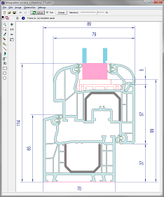
Example of window frame analysis.
Left: geometry is “filled” with materials using the Bitmap Editor.
Right: Calculated temperatures and heat flows.
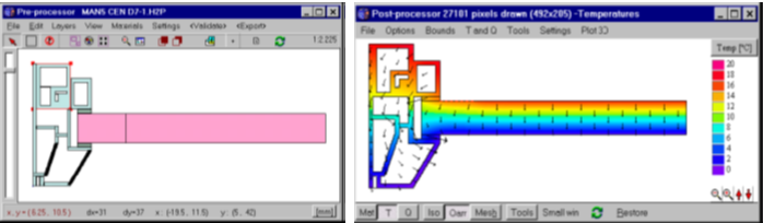
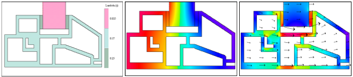
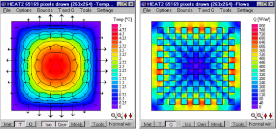
Slab on the ground. Pre-processor (left). Post-processor showing temperatures (middle) and heat flow intensities (right) indicating a large thermal bridge effect (red color). Heat flow arrays are also shown.
 Window frame analysis. Pre-processor (left) and post-processor (right) showing temperatures and heat flow arrays.
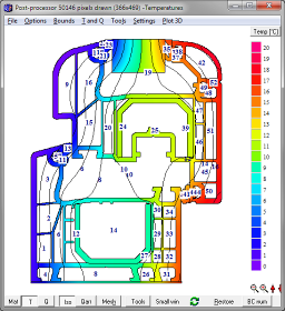
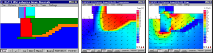
 Window frame analysis. Post-processor showing materials (left), temperatures (middle) and heat flow intensities and array (right)
 Left
Left
Window frame with 11 cavities with radiation and convection calculated according to ISO 10077.
Right
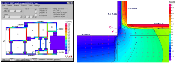
Slab on the ground. Detail of wall/floor/ground connection. Temperatures and heat flow arrays.
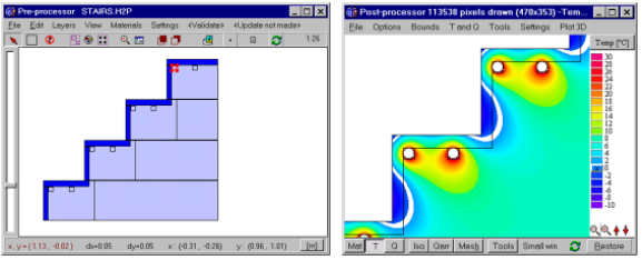 Stairs heated by heating pipes (frost protection). Pre-processor (left) and post-processor (right) showing temperatures. Isotherm T=0 shown as white band.
 Floor heating. Pre-processor showing temperatures and isotherms (left), heat flow intensities and arrays (middle) and temperatures in 3D (right).
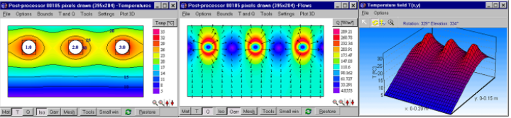
 85 heat sources of 1 W/m placed in a checkerboard pattern. Pre-processor showing temperatures and isotherms (left), heat flow intensities and arrays (right).
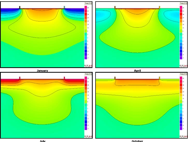 Yearly temperature variation beneath a slab on the ground. The outdoor temperatures has a maximum of +23 °C and a minimum of -7 °C, see function 1 defined as below
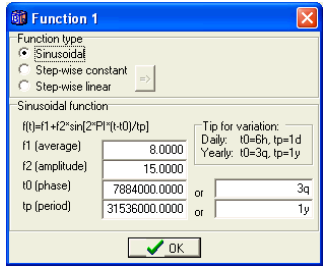 Sinusoidal variation for outdoor temperature.
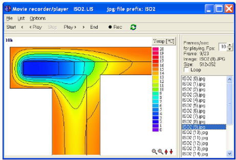 The Movie Maker captures graphical output data, such as temperatures, isotherms, and heat flows and makes a standard AVI-file.
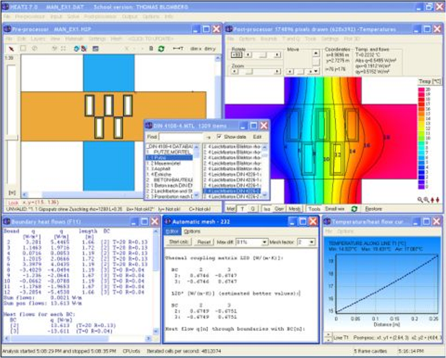
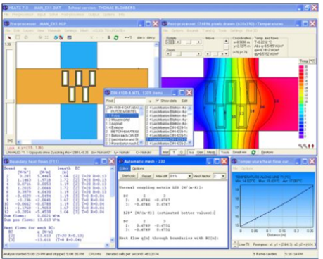 HEAT2 user interface.
Tips for reading for beginners: For a quick start read Chapter 4 (pages 23-27) in Manual HEAT2 5.0. The example in chapter 8 (pages 117-121) would also give a short introduction. After this, look at the update manuals for HEAT2 6.0, HEAT2 7.0, etc. Also see the EN ISO test cases: [ISO 10211 & 10077-2 validation test cases].
Update manual HEAT2 8 (PDF), 2011
Update manual HEAT2 7 (PDF), 2006
German: Updatehandbuch HEAT2 7 (PDF), 2006
The theory is described in this thesis.
Below are some frequently asked questions for HEAT2 and HEAT3.
General
- My transient calculation takes long time. Why?
A.
You may have entered a wrong volumetric heat capacity. It should be around 1E5-1E6 J/(m3,K) (that is 0.001-1 MJ/(m3,K). Note that the volumetric heat capacity is the density times the specific heat capacity. In a STEADY-STATE calculation, the heat capacities do not matter.
Another possibility is that you have very small numerical cells. It is the ratio volumetric heat capacity divided by the thermal conductivity that determines the stable time-step. This means that it is often steel (and other materials with a high ratio) that gives the lowest time-step.
The following table shows some material. A transient simulation using steel may e.g. take 55 times longer compared with using brick (3.3/0.05=55).
Try also to change the over-relaxation coefficient and see if the flows changes faster during the simulation. The optimum coefficient is often 1.8-2.0. Use a large over-relaxation coefficient (1.95-2.0, see manual) when there is a high ratio between the thermal conductivities. Another tip is to start with the expected temperature in each given box (especial the areas with high conductivity).
_______
- Can I run several problems in a batch mode?
A.
Batch mode is not direct supported. But one way to run different problems is to start several instances of HEAT2/HEAT3 solving the different problems simultaneously. This requires enough RAM on your system.
_______
Q.
We would like to simulate a room with an attached conservatory. Is it possible to simulate the solar radiation or a test reference year ? – is it possible to work with more than one function or to add a factor? (e.g. conservatory 15 – 30°C, room 20 – 25°C(half amplitude)) is it possible to combine heat with other programs e.g. that calculate air flow or simulate large buildings/e. g. IES FACET, ESP, TRNSYS….)? thanks to your help.
A.
The prescribed boundary conditions may only be temperature with surface resistance, or a given heat flow. You can simulate a reference year with temperatures (sinus or stepwise), but not with solar radiation. HEAT3 has only one function, but HEAT2 can handle three. No interfaces to other programs have been done.
_______
- I am very impressed with the capabilities of your software. I am interested in using this package for analysis of a small system enclosure with various layers of insulating materials. I have several questions however:
1) Can you create your own materials in the library with custom properties?
2) Can you work small physical scale models as well as large scale (building) models?
3) With purchase of the Heat 2 /3 package, what is the version upgrade /support policy?
4) Can temperature and heat sources time dependent data be input from a file?
5) How is convection boundary layer handled?
A.
1. Yes, open the material editor (item Materials/Edit materials in the pre-processor, or double click on any material in the pick list). Use Edit/Insert record to add a material. See the on-line manual for more info.The coming version 4 of HEAT3 will use the same material file format as HEAT2.
- There are really no physical scale limitations (lengths could be e.g.between 1E-5 and 1E5 meters).
- Seebuildingphysics.comfor info.
- In HEAT2, boundary conditions, heat sources and internal areas of a specified temperature may be a function in time (sinus, step-wise constant or step-wise linear). The function editor (text file with step-wise constant or step-wise linear values) can import different formats, data may be cut and pasted from e.g Excel. See the manuals for more info.
- A surface resistance coefficient (inverted heat transfer coefficient) is given as a fix value.
_______
- I am interested in a HEAT3-type of software program but for cylindrical co-ordinates. Do you have one that would solve a simple-geometry 3-dimensional heat conduction problem?
- We only have an older dos-program for transient and steady-state heat transfer in cylindrical co-ordinates. The program will run on Windows 95/98 in dos mode.
_______
- We have problems opening files created with an earlier version of Heat 2. In particular we are unable to use / modify models within the pre-processor integrated in current version 5.0. How can we overcome this problem? Your earliest reply would be appreciated very much.
- The data files of versions before 5.0 do not contain information that is needed by the HEAT2 5.0 pre-processor. The pre-processor can only be used to specify new problems with. You can load older files but only work with them in text-style format.
Simulation/Performance
Q.
I quickly tested your 3D conduction software Heat3 downloaded March 8, 2000: I like the interface (text file oriented but with immediate graphics update), but I have great concerns about the limitations.
1) In my typical application I have a BGA IC (ball grid array integrated circuit) or flip chip, in electronic application, where in X axis I may have 13 solder balls (could be 20 as well, same in Y direction), each ball (small sphere) being represented for instance by 4 cells in X (sphere represented by box), and they are spaced by eg 4 cells also.
If I understand correctly, for 20 balls I will need 40 segments in X at least (one segment at least for each material transition, right ?). There may be 50 to 200 such solder balls in my model in the XY plane. Defining the geometry for repetitive structures should be easy since I can write a small C program to generate the DAT file. My PC has 2 GB RAM so from what you said I expect that the RAM only will limit the cell number to about 400 in X,Y,Z.
2) Boundary conditions in Heat3 can be defined with functions, but only function of time it seems, I would have been interested in BC where the thermal resistance toward ambient (or flux) is a function of temperature, such as: Q in Watt = dS x Constant x ( (T+273.15)^4 – Constant) + dS x Constant x T^0.25 (where dS is cell area). Steady-state only. Did you receive any request from other customers for such a feature, and would it be hard to implement ?
3) I may use dimensions as small as some microns (silicon chip…). Is there some round-off truncation in the software which could lead to errors for small dimensions like these ?
A.
1. Yes, you will need n*2-1 segments where n is the number of boxes. 200 boxes will use 399 segments. A special version may be used:
-A. 400 maximum segments, 250 maximum boxes, Nx=Ny=Nz=200 (about 260 RAM is required)
-B. 400 maximum segments, 250 maximum boxes, Nx=Ny=Nz=400 (about 2 GB RAM is required)
The amount of RAM is roughly N*32+10 MB. Note that the amount of cells does not have to be equal in all directions. E.g. Nx=500, Ny=500, Nz=50 would only require about 410 MB RAM. Feel free to specify your own data fields.
The text editor can hold 16 MB of text (160 characters per row would give a maximum number of rows of 100 000) so this should present no problem for you.
- It would be possible to implement a heat flux according to you formula. No other customer has requested this kind of boundary condition.
- I think it will be ok, but I cannot answer this question since problems may arise with a large amount of cells. See answer 3.
_______
- I thought that I had managed to do 3D transient calculations to look at temperatures at the corner of a footing, but it seems I was mistaken! I was puzzled by the results, because temperatures that should have agreed with 2D transient calculations did not by a margin of several degrees. When I went back to look at my input, I found that I had forgotten to change the capacities – all the materials were set at 10E-6 (nevertheless, it had taken most of 4 days to do the calculation). When corrected, these values slowed things down amazingly! I tried to simplify, but even with fewer cells the difficulty persists.
Rather than fumble about, I decided to run your SLAB file with a mean temperature of 9.4, a period of 1 year, amplitude of 10, and phase of 0, after an initial steady state run without modification. I changed only the one boundary condition. Running for 59m19s of CPU time, ICPS=185425, I managed to simulate only 1m22s of virtual time. That means (unless the relationship between real and virtual time is non-linear) that temperatures after 10 years would take only 600 years or so to predict! My own models, even when greatly simplified, were taking similar amounts of time. Is this reasonable, or should I be looking for something wrong with my equipment? I am running under Windows 2000 Professional on an AMD Athlon 950 machine.
If my equipment is performing to expectation, I must abandon the idea of doing 3D transient calculations to compare temperatures at external corners with and without insulation, unless you can see a way. With very low thermal capacities, the calculations are within the realm of the possible, but I assume the results are spurious. Can you confirm this? I’m not interested in flow as much as temperature.
My next idea is to use 2D transient calculations first, and then find an exterior temperature that produces the annual minimum footing temperature midway between corners with a 3D steady state calculation. Would it be reasonable to assume that conditions at the corner predicted by the same means would also approximate the annual minimum?
As always, any suggestions will be most welcome.
- The reason that it took so long time for the slab example is that the heat capacities are not set to correct values for this transient case. They are all 1.0 here which may be a factor 1e6 or so wrong. I tried the example with the heat capacities set to 1e6 for all materials just to get an idea of the simulation time (the value for the insulation is of course not so good). It took me a CPU time of 45 min to simulate one year (ICPS 720 000).
My machine is a PIII 500 MHz. Your PC should be almost twice as fast (I guess about 1.9 times). I am a bit puzzled that you get an ICPS (Iterated cells per second) of only 185425. It should be about 1.2 million if we look at the clock rate for the PIII and Athlon (I have made some test on a Athlon 850 which was 1.8 times faster then my PIII 500 for some HEAT2 calculations). Maybe you have other resident programs (Norton utilities?) that takes up CPU-time.
What time does it take to solve the enclosed HEAT2 problem “bench.dat” on your PC? Just load the file and press F9. It takes 29 sec on my PC, 2678 iterations, N=25600 cells, HEAT2 ICPS=2.36 million. There are some additional benchmarks in the manuals.
If you are interested in temperatures close to the ground at the corners (maybe within 1 meters from the ground surface or so) I think that true 3D calculations are best. There might exist some 2D tricks in certain case, but I am not familiar with those.
_______
Q.
I have not tinkered much with the Slab Demo, but perhaps some suggestions will be of use. If I understand correctly, the insulation is only under the building, not around the perimeter extending beyond the building. Because of concerns about frost, this model is of little use in our climate. The annual heat flow from the building is of interest, of course, but I also need assurance that the ground is not freezing under the building.
Using Heat3, I am going to try looking into the effects of a combination of insulation under slab on grade, with perimeter insulation on a horizontal plane in the ground extending beyond the building, including a building corner. (Given the speed of my computer, and my age, I wonder what is the probability of completing this task in my lifetime?)
To speed the process up, I’ve started with a 2 dimensional model, steady state, with the exterior temperature at annual average, to get a starting temperature field. I am now doing a transient run, with f1=0 (i.e. starting with August, more or less), to stop at a month. I am starting with August in hopes of minimizing differences between steady state and transient temperature fields. It is clear from the initial progress that to run a full month will take a long time! (So far, more than an hour to do 10s of model time.) I can speed this up somewhat by removing device drivers and background processes, and refraining from doing other tasks, but this seems a faint hope. Can you suggest ways to get a less accurate answer in less time?
The full program I am trying to follow is:
- What minimum temperature does the footing bearing surface experience during the annual cycle, using a 2D transient model? (At the moment, I’m doing this with Heat3 and a 1 cell vertical slice from the 3D model with all of the sub-grade insulation having the same properties as the ground, and the number of cells reduced.
- With a full 3D model, under the same conditions, what is the temperature under the footing at the corner, and how far back along the wall does the influence of the corner extend?
- What steady state exterior temperature will produce the same temperature at the base of the footing as in step 1, in 2D?
- In 3D steady state, will the same exterior temperature produce the same corner temperature field as in step 2?
- In 2D steady state, if insulation is added under the slab, what additional insulation is needed outside the building to restore the footing to the same temperature as in 3?
- In 3D steady state, with insulation under the slab, what augmentation at the corner is needed to restore it to the same temperature as in step 2?
Any suggestions you’d like to share will be welcome.
A.
Perhaps chapter 11 “A few tips” in the HEAT2 manual may help you. Most of it applies to 3D cases as well. You should try to use a fast computer with a modern Pentium or a Athlon CPU. Using larger numerical cells will increase the time-step but also increase the numerical error.
When I have problems of this kind with frost heave, I usually start from the steady-state temperature (with the average outdoor mean value) and then continue with transient calculations with a sinusoidal maybe 3-5 years until more or less the same variation is reached. After that I apply a sudden cold-spell (e.g. -18 degC) for 1 or 2 weeks and look at the isotherms under or near the house. A rule of “Swedish thumb” is that the zero degree isotherm must not reach below/under a 45 degree line that goes under and out from the side of the house. However if the soil is not sensible for frost heave the zero isotherm may go beneath the house. The corner (3D) is normally used when looking at worst-case scenario. The second part of the German report you got deals with added horizontal insulation outside the corner of a house.
Even if transient calculations take time, I think it is better to do this than to try to approximate the temperature field close to the slab with steady-state calculations.
_______
- Continued from last topic…
I’ll re-read the manual in case there’s something I missed. My present computer has a Pentium Model 8 23 with math support on chip @ 233 MHz with 64 megs of RAM running WIN95 4.00.950B. If I cannot solve this problem in a reasonable time without a faster one, I’ll get one. However, I don’t want to find out that even then, the problem is too time consuming. Have you any idea what would be the minimum? Are there architectural differences between my Pentium and more recent models that make a difference, apart from clock speed? Would more memory help (my guess is not)?
I started on the same path anyway, although I failed on the first attempt to change the boundary condition to “function”, an error I’m not likely to repeat. A soils consultant has suggested soil with conductivity of 1.4 W/mK and capacity of 2.35 MJ/m3K to represent the local clay till. The current state of the art in rules of thumb here is that next to a heated building, a foundation depth of 1.2 m below grade is adequate. There is a similar rule for isolated foundations, but the depth eludes me at the moment. Since, if the soil is moist, the advance of the 0 deg C isotherm (and it’s subsequent retreat) would be much less rapid than the transient calculation will indicate (due to heat of fusion). I still intend to assume that even if freezing is indicated within the splay of the foundation by the transient calculation, that things are OK, since these foundations perform adequately in fact. Moisture (increasing capacity), freezing, insulation due to snow, solar heat, and surface resistance are all factors that are not fully accounted for ,and that tend to make the transient calculation conservative.
Thank you for reminding me of the bearing splay of foundations – I know this but had not related it to this context. Unfortunately, no one has volunteered to translate the German paper for me.
I understand and appreciate your caution, although I may not follow your sage advice in this regard. Even with a much faster computer, I wonder how long it might take?
A.
Here are some data about numerical performance.
HEAT2 and HEAT3 optimize performance for Pentium II and III (and probably the same for P4). A Pentium III 500 will probably be 4-5 times faster than your Pentium 233. See chapter 7 in the HEAT2 manual for more info.
The clock rate is the most important factor for PII and III systems, i.e a PIII running on 1 GHz is twice as fast as a 500 MHz CPU for calculations with HEAT2 and HEAT3. Adding more memory will not increase sepeed. 64 MB of RAM is sufficient.
It should be sufficient to run the 3D frost heave problem for a simulation period of 3-5 years overnight. You will have to elaborate on the numerical mesh and not choose a too dense grid. You might end up with a 5% (or even 10%) numerical error but this should suffice. After all, the uncertainty of the soil properties are probably much higher than this (in addition you have all the conservative factors you mention below). You can estimate the numerical error by doing two fast steady-state calculations, one with the mesh you intend to use in the transient calculations and one with a denser grid that gives a “true” value for heat flows/temperatures. You then have an indication of your numerical error for the used mesh in the transient calculation. I think that this error will give reults on the safe side; a sudden cold spell will give a larger penetration depth using a less dense grid compare with a more dense grid. But since the outdoor temperature varies a few years sinusoidally, this may not be true. Let me know if you find out anything about this.
_______
Q:
I am calculating the enclosed cladding frame edge for a large office tower in Saudi Arabia on HEAT3. The problem is TOP URGENT as the erection of the cladding is blocked until the U-value calculation is submitted. Every day costs my customer a penalty sum.
I have made the enclosed input. The input would satisfy the HEAT3-50 conditions. When steady state solving on HEAT3-50 or HEAT3-c, I receive an error message: Too many internal cells: (2326) Maximum = 1000. In the manual no restrictions are made for a number of internal cells. The expression ‘internal cells’ is not defined, so I do not know how to alter this number.
Please help us immediately to solve this problem. For your immediate collaboration we thank you very much.
A.
Internal cells are those that meet in an inward bent corner. It gets very seldom over the limit of 1000. Either you must have a very complex geometry or the input is not quite right. This means that the number of cells along a corner that is bent inwards exceeds the maximum number 1000. The info log shows also the message:
“.. Seeking cells at internal corners… Found=57 OK”
In the future you may also want versions with more cells. The limit is the PC memory size (RAM). The following list shows some examples for HEAT3:
- -1.7 million (120*120*120) requires about 60 MB RAM (a pc with 80 MB RAM is recommended)
- -3.4 million (150*150*150) requires about 120 MB RAM (a pc with 128 MB RAM is recommended)
- -8 million (200*200*200) requires about 250 MB RAM (a pc with 256 MB RAM is recommended)
- -16 million requires about 500 MB RAM (a pc with 512 MB RAM is recommended) etc.
Note that the amount of cells in the three directions does not have to be equal.
_______
Q.
I have tested your heat2 program and have a question about it: Why is the unit of the heat capacity C MJ/m3K and not kJ/kgK ? And how can I convert?
A.
The volumetric heat capacity C is defined by the specific heat capacity cp times the density.
_______
Q.
In these days I’m involved with a study on cruise vessels’ passengers cabins vs. eventual fire. Our aim is to have a cabin model with which execute a 3D forecastle of temperature inside the cabin in different fire situations. Has your Company some Software product fit to my needs? Have you ever used it for this particular target? Could you tell me the prices of this software? Looking forward to your answer I’m sending you my Best Regards.
A.
Our 3D model HEAT3 does not account for radiation exchange. It is a model for pure heat conduction. It may be used in your case to see how the interior surface temperature varies in time after a sudden raise of the external temperature (on the other side of the wall). Note that the material properties are constant (not a function of temperature).
Standards
Q.
As our company is mainly involved in design, fabrication and installation of bespoke metal/glass facades and roofs, very often we have to deal with high performance glass, designed as retained glazing, point supported glazing and/or silicone structural glazing. In conjunction with that, can you please advise us, whether it is possible to model glass panels with low emission coatings, sun protection coatings and/or ceramic frits within Heat 2 5.0 ? Please take also into account that coatings may be on the outside or towards the cavity of the insulated glass units? Your earliest reply would be appreciated very much.
A.
Thank you for your email. HEAT2 does not model heat exchange by radiation for outside surfaces. Only long-wave radiative calculations within a cavity may be done. For more information about features for HEAT2 see our on-line manual.
There are often different standards in different countries and you should normally follow the one adopted by Germany. Here is a list of some related ISO standards.
- EN 673 Glass in building Determination of thermal transmittance (U-value) – Calculation method
- prEN 12519 Doors and windows – Terminology
- EN ISO 6946 Building components and building elements Thermal resistance and thermal transmittance Calculation method
- EN ISO 7345 Thermal insulation – Physical quantities and definitions
- EN ISO 10211-1 Thermal bridges in building constructions – Heat flows and surface temperatures Part 1: General calculation methods
- prEN ISO 10211-2 Thermal bridges in building construction Heat flows and surface temperatures Part 2: Calculation of linear thermal bridges
- ISO 10292 Glas in building Calculation of steady-state U-values (thermal transmittance) of multiple glazing
HEAT2 5.0 has also possibilities to calculate heat transfer within frame cavities according to the current proposed standard prCEN/ISO/TC 89/WG7, document prEN10077-2 ( (Thermal performance of windows, doors and shutters – Calculation of thermal transmittance – Part 2: Numerical method for frames).
_______
- We are looking to verify the prediction of heat transfer of our in-house program a colleague and myself have developed a finite element based program for structural and transient analysis. We need to verify our 3-D computation of heat transfer. My discussion with Dr. X of IRC brought your HEAT3 development to my attention. It would be useful if you can give or guide us of some examples for our verifications. We are also looking for layered composite examples. Your help in this regard will be very much appreciated.
A.
HEAT2 and HEAT3 meet the standard requirements in EN ISO 10211-1 (“Thermal bridges in building construction – Heat flows and surface temperatures – Part1: General calculation methods”). The document contains three calculation cases that have been validated using HEAT2 and HEAT3. Two of them are covered in the manuals for HEAT2 and HEAT3, see page 135 (HEAT2) and page 68 (HEAT3). HEAT2 and HEAT3 confirm to the standard to be classified as a high-precision method according to the standard. You can validate your own model using the same input.
_______
Q.
I have a question to ‘new’ European standard: Is it possible to calculate ‘linear thermal transmittance’ (EN ISO 14683) at thermal bridges with HEAT-program?
A.
Yes, the linear thermal transmittance coefficient may be calculated with HEAT2 (2D) and HEAT3 (3D).
_______
Q.
In evaluating your calculation program HEAT2, we checked the manual example (p. 166) of the CEN aluminum window frame (example 1 in prEN ISO 10077-2:1998). Your drawing is slightly different from the one in 10077-2:1998 (dxf in attachment).
If the drawings changed for version 10077-2:2000, please send us the result for total heat flux (W/m) and U-value of the frame, as mentioned in the new version of the standard (which I don’t have).
If the drawings didn’t change, is it possible to send us the intermediate and final results for our dxf-attachment? Thanks for helping us in the evaluation of your calculation program.
A.
Thank you for your email. I believe that most of the examples have different geometry in 10077-2:2000 compare to 10077-2:1998. The heat flow for example D1 becomes 11 W/m (0.55 /m,K). The U-value becomes 3.2 W/m2,K. I think that the heat flow for the old geometry (10077-:1998) was 11.2 W/m. Let me know if you have further questions about HEAT2/HEAT3.
Graphics
Q.
1. Is there a way I have not found to save graphic settings in Heat 2 and 3?
When I prepare bitmap images to compare to each other, I need to get back to the same viewpoint, zoom, scale, isotherm, rotation, etc. settings as previous sessions to create comparable images for conditions I did not think of before. Every time I close a file, these settings are lost. They cannot be retrieved either, in the case of click and drag settings, with adequate accuracy. I need to open a DAT file, load a PSE file, and then ….? to get the same image I had in a previous session. Even the ability to open a DAT, and then load PSE files one after another without resetting the graphics would be very helpful. Please tell me I’m being stupid again, and how to do this!
- When images are saved as BMPs, only MS Paint is able to open them. Graphic Workshop, Adobe Photoshop, MS Powerpoint, and other programs I’ve tried to use them with (and which normally open BMP files without problems) all report that they cannot be parsed, are damaged, or they open the file and display garbage. The number of colors is set to 254 (why won’t Heat accept 256?) and I believe some of the other programs can handle up to 24-bit depth files. Any idea what’s the problem?
A.
1. No, there is unfortunately no way to save the desk-top. One tip in HEAT3 is to count the number of times you press the keys q, w, e to rotate the picture.
2.
I had no problem to open and import a BMP-file saved by HEAT2 into Word 2000 and Powerpoint 2000.
I could however not import it into an older version of Adobe Photoshop (ver 5.5). There are two simple solutions: 1. Cut the image to the clipboard (see the HEAT2 manual, Section 5.18.3) or 2. open the bmp-files in MS Paint and save them as jpg or tif that can be imported into other programs.
Regarding the colors; maybe you are using 256 colors in Windows? It should be set to at least 65 000 (“Hi color (16-bit)”). Actually, the 254 value denotes the number of shades in HEAT2 that are chosen from these 65 000 (or more) colors. It would make any sense to use more colors since it is hard to see the difference between the shades (at least with the false color representation I use). If you set the number of colors to 100 in the scale option menu, you will hardly see the difference.
Q.
Is there a possibility to show two or more charts of recorded “T, points” all at once?
A.
Yes, do as follows:
1. In the record window choose menu item “Graphics” for column “1”. This will open the chart window with series1.
2. Go to Options/Edit chart in the chart window.
3. Go to the “Series” tab and press the “Clone” tab. Series 2 will now be a copy of series 1.
4. Change the “show graphics” in the record window to column “2”. Now, the shown series 1 is the default series (column number 2 now). The second shown series is the old copy of series 1 (column number 1).
In this way you can copy each default series to the “stack”.
Example (see figure below):
E.g three defined columns with temperature:
Column 1. Show graphics for this column. Copy this to stack with the clone commando. Change color to orange.
Column 2. Show graphics for this column. Copy this to stack with the clone commando. Change color to green.
Show data for column 3. This will show the picture below.
Note that the clones must be deleted by hand in the chart editor when new values are recalculated.

Current version of HEAT2 is 10.2
Use the update function (menu item Info/Check for updates) to see if there are any updates. This will show the download link to the setup program. Note that you can also use the (same) download link you got in the order email since it always will contain the most recent version.
For detailed info please see Appendix A in
https://buildingphysics.com/manuals/HEAT2_10_update.pdf
Version 10.2
March 21, 2024
-
The license manager has been updated with many performance improvements.
-
HEAT2 now install material files (and some other files) to the common folder C: Users Public Documents BLOCON HEAT2 10 by default so that the files can be shared by different users. See also Section 1.5 “Installation”.
-
Windows theme now default at start-up. This can be changed in menu item Options/Themes.
-
Modern design for the open/save file dialog.
-
New version for setup program.
-
Bug for loading old files saved with v8 fixed.
-
The font for materials heading in the post-processor can be changed, see menu item Settings/text font in right panel in the post-processor.
Version 10.13
June 11, 2020
-
This update contains a fix for a rare calculation type where temperature dependent material properties have been used, see chapter two in
https://buildingphysics.com/manuals/HEAT2_9_update.pdfThe bug was recently reported by a user and it is only affecting the case
“Type 2, piecewise linear volumetric heat capacity and thermal conductivity”In some cases where EITHER the volumetric heat capacity OR the thermal conductivity were depending on temperature, the resulting calculated temperatures may have an error depending on the input range for temperatures.
Therefore we suggest that you re-calculate your old cases if this specific case has been used.
If BOTH the volumetric heat capacity AND the thermal conductivity were depending on temperature the results in the old versions are ok.
If you have used “Type 1, Freezing of soil”, or the predefined material for steel named “TDEP_STEEL”, all calculations using older versions are also ok.
Please use your original download link that you earlier received by email to download and install the latest version.
For floating licenses: please download and install the latest version for each client (use your old download link that is updated).
If you have any questions please contact us at info@blocon.se.
Version 10.12b
April 23, 2017
- For admins/superusers: It is now possible to silently install, uninstall, activate, and deactivate HEAT2 using a command line in a batch-file, see
buildingphysics.com/download/silent_heat2.pdf
Version 10.12
April 14, 2017:
- Compatibility with Windows 10 “Creators update” added.
Earlier versions of HEAT2 will not start if your OS is updated to Windows 10 “Creators update”.
There is however a quick fix that will make old versions of HEAT2 run under this OS:
Go to folder C:Program Files (x86)BLOCONHEAT2_v10.11, right-click “HEAT2_v10_11.exe” and choose
Properties. In the Compatibility tab, change “Compatibility mode” to “Windows 7”. - New version of TurboActivate (4.0.9.6).* IMPORTANT WHEN YOU INSTALL V10.12 *:
If you have any old versions prior to HEAT2 v10.12 on the PC you need to uninstall them first in the
control panel before continuing.
Version 10.11 update
August 30, 2016
- Compatibility with Windows 10 Anniversary added.
Version 10.1 update
July 25, 2016
- New look of file open/save dialogs
- Preview possible for Dxf/Dwg-files in the Cad import open file dialog
- Fixed problem: clicking in the post-processor menu sometimes froze the image for a short while
- Fixed problem: some windows were earlier hidden when toggling between HEAT2 and other applications
- Fixed problem: “cannot open clipboard: access denied” sometimes came when pasting objects in pre-processor
- Max value for coordinates for ”Input/Initial Temperatures” raised from 250 to 32767
- Max value for coordinates for ”Input/Resistances” raised from 250 to 32767
Version 10.03 update
June 7, 2016
- Maximum value for coordinates for ”Areas with internal modifications” raised from 250 to 32767
- The small ”squares” indicating current material color were not updated when ”Themes” were applied. (The squares are shown in Material pick list (at upper right), Pre-processor (at lower left), Bitmap editor (black and white squares on the tool bar), and in the Tool menu in the Bitmap editor).
Version 10.02 update
March 10, 2016
- Bug fix for material editor that “froze” on certain systems.
Old versions:
HEAT2 9.05
Use the update function (menu item Info/Check for updates) to see if there are any updates. This will show the download link to the setup program. Note that you can also use the (same) download link you got in the order email since it always will contain the most recent version.
Version 9.05 update
June 11, 2020
· This update contains a fix for a rare calculation type where temperature dependent material properties have been used, see chapter two in
https://buildingphysics.com/manuals/HEAT2_9_update.pdf
The bug was recently reported by a user and it is only affecting the case
“Type 2, piecewise linear volumetric heat capacity and thermal conductivity”
In some cases where EITHER the volumetric heat capacity OR the thermal conductivity were depending on temperature, the resulting calculated temperatures may have an error depending on the input range for temperatures.
Therefore we suggest that you re-calculate your old cases if this specific case has been used.
If BOTH the volumetric heat capacity AND the thermal conductivity were depending on temperature the results in the old versions are ok.
If you have used “Type 1, Freezing of soil”, or the predefined material for steel named “TDEP_STEEL”, all calculations using older versions are also ok.
Please use your original download link that you earlier received by email to download and install the latest version.
For floating licenses: please download and install the latest version for each client (use your old download link that is updated).
If you have any questions please contact us at info@blocon.se.
· Compatibility with Windows 10 Anniversary added.
(If “Stop calculation” button does not respond this update will fix it).
· New license manager (you must uninstall v9.04 and earlier versions before installing this update)
· Other small improvements
Version 9.04 update
Feb 4, 2016
- The modification “Pipe (heat source)” could not be used for transient enthalpy calculations where phase change was occurring in previous version. This is now added.
- Fix for randomly occurring “floating point error” on Windows 7 when calculation was made using menu item “Automatic mesh and L2D”. (One user has reported this error.)
Version 9.03 update
March 18, 2015
- A few font fixes.
Version 9.02 update
Jan 15, 2015
- Improved license management.
Version 9.01 update
Jan 8, 2015
- Bitmap image resizing and resampling improved.
Version 8.1 update
April 15, 2015:
- Better adaption to Windows Vista, Windows 7 and Windows 8
- Several instances of HEAT2 can now be started and active at the same time. This will allow you to work (input and solve) multiple cases at the same time. Solving e.g. 3-4 cases parallel on a CPU with four cores, or 5-6 cases on a CPU with 6 cores should be very efficient.
- Now multilingual + many other smaller improvements.
- New improved license management system.Your “old” license key for HEAT2 v8.0-v8.03 needs to be converted to a new product key for v8.1. This can be made here: Generate new product key.
To upgrade your old license of HEAT2 v8.0-v8.03 to v8.1 please use the update function in HEAT2 (menu item ”Info/Check for updates”).
Version 8.03 update
Aug 1, 2011:
- Improved input on the length panel at the bottom of the pre-processor.
Version 8.02 update
July 21, 2011:
- If a polygon point was drawn to close to another point, it would sometimes be missing.
This is now fixed.
Version 8.01 update
June 20, 2011:
- The error message “This material file is not allowed in demo version” was sometimes shown.
This is now fixed.
Version 7.1 update
2009-03-30:
- Fixed error message ”HEAT2 is registered but ActiveX does not exists”. This alert came in some cases for a user without admin rights running HEAT2 under Vista and XP.
- Calculation of psi-factors: HEAT2 assumed for some cases that the indoor climate were placed on the left side of a wall/roof leading to that legends for external/internal lengths ”L(i)” and “L(e)” sometimes were switched.
- Frame cavities:calculations for frame cavities gave an overestimation of a few percent for the heat flow due to radiation when the cavity was enclosed by surfaces with temperatures below zero.
- Recorder: fixed label “Q, point (x,Y) [W/m?]” => “Q, point (x,Y) [W/m2]”.
- System info: “Available virtual memory” was negative if RAM size was above 2 GB.
- Options for steady-state: options for optimization of over-relaxation and numerical scheme are now saved to file.
- Function steps editor: “Paste from clipboard” added to menu.
EN ISO 10211:2007
HEAT2 is validated to conform both two-dimensional cases of ISO 10211:2007, Annex A.
HEAT3 is validated to conform all 4 cases of ISO 10211:2007, Annex A, for three-dimensional calculation programs.
See this PDF-file for results:
buildingphysics.com/download/iso/ISO_10211_HEAT2_HEAT3.pdf (1,2 MB PDF)
The HEAT2 data files may be downloaded here :
buildingphysics.com/download/iso/HEAT2_7_files_iso10211.zip (5 kB zip-file)
The HEAT3 data files may be downloaded here :
buildingphysics.com/download/iso/HEAT3_5_files_iso10211.zip (12 kB zip-file)
EN ISO 10077-2
HEAT2 is validated to conform all 10 cases of ISO 10077-2. See this PDF-file for results:
buildingphysics.com/download/iso/ISO_10077_HEAT2.pdf (1,8 MB PDF)
The HEAT2 data files may be downloaded here :
buildingphysics.com/download/iso/HEAT2_7_files_iso10077.zip (50 kB zip-file)
Danvak has courses (info in Danish but may give courses in English):
https://danvak.dk/aktiviteter/linjetabsberegning-med-heat2-grundkursus/
https://danvak.dk/aktiviteter/linjetabsberegning-med-heat2-udvidet-kursus/
Please contact info@svensk-energiutbildning.se for courses in English/Swedish:
https://svensk-energiutbildning.se/koldbryggor-i-energiberakning-och-projektering/
List of 1100+ consultants and universities in 25+ countries that use HEAT2/HEAT3:
List of 150+ universities and research institutes in 25+ countries that uses HEAT2/HEAT3:
Download light version of HEAT2 10
Please fill in the following form. A password is required to install the program. The download link and password will be sent immediately to your email